Directional derivatives and JAX

Feb 8, 2022 · 4 min read

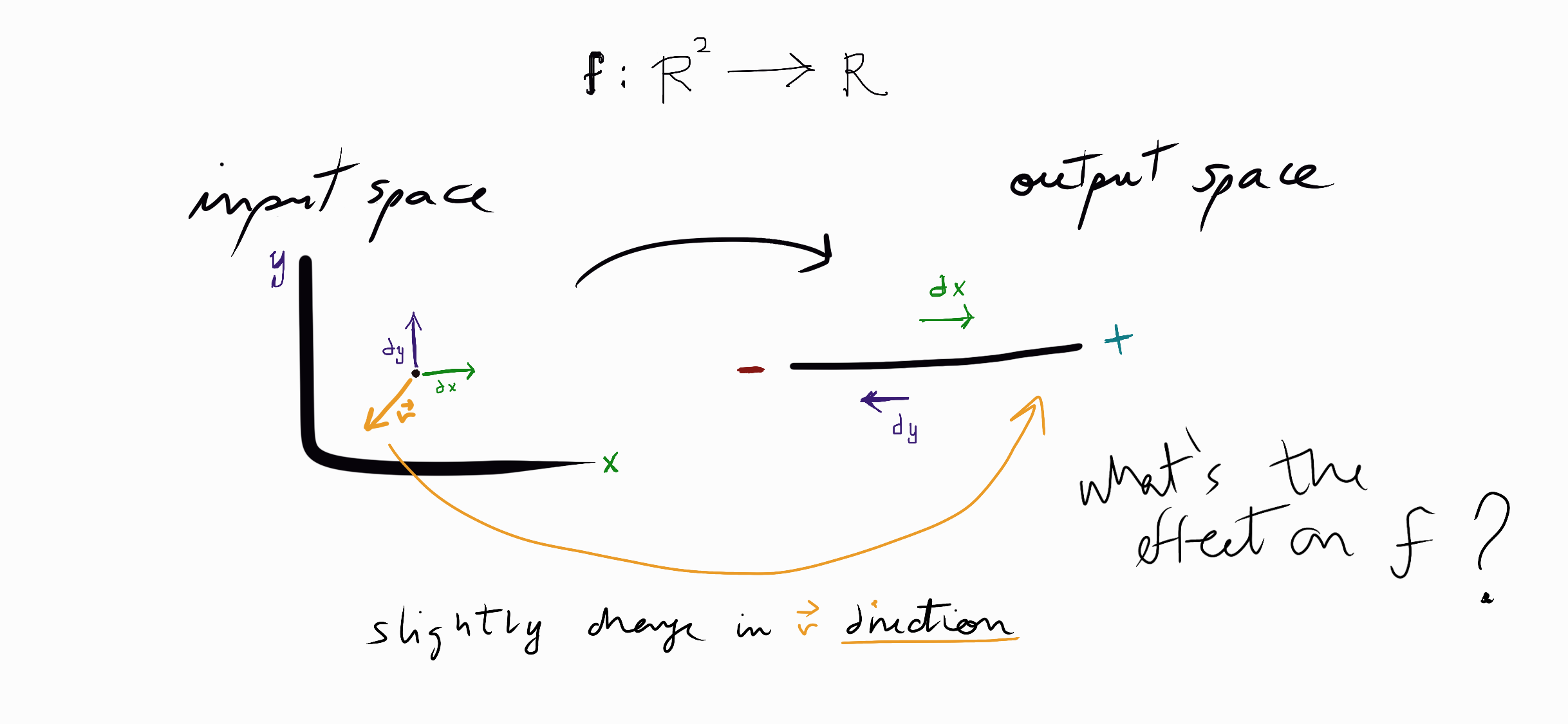
Directional derivatives are the conceptual tool to measure the effect on a function by changing the input in any direction within the input space. It's possible to compute the directional derivatives using the jacobian-vector product, implemented by the automatic differentiation JAX library.

Partial derivatives $\partial f / \partial x_{i}$ give us the rate of change if we slightly modify the ith element of the input vector $𝐱$ by h, letting the rest constant.

\frac{\partial f}{\partial x_{1}} = l i m_{h \to 0} \frac{f (x_{1} + h, x_{2}, \dots, x_{n}) - f (𝐱)}{h} parsing error: new line command not allowed in current environment
╭─► context:
│
│… x})}{h}
│ \\
│ \vdots
│ \\
│ \f
│ ^^
╰─── ⋮ parsing error: new line command not allowed in current environment
╭─► context:
│
│…\
│ \vdots
│ \\
│ \frac{\parti
│ ^^^^^^^^^^^^
╰───────────── \frac{\partial f}{\partial x_{n}} = l i m_{h \to 0} \frac{f (x_{1}, x_{2}, \dots, x_{n} + h) - f (𝐱)}{h}

The above definition can be more compactly using vector notation.

\frac{\partial f}{\partial x_{i}} (𝐱_{𝟎}) = l i m_{h \to 0} \frac{f (𝐱_{𝟎} + h 𝐞_{𝐢}) - f (𝐱_{𝟎})}{h}

The $e_{i}$ vector represents a unit vector in the direction of $i$ with the same number of dimensions that $𝐱_{𝟎}$ . The only element of $e_{i}$ different from 0 is the ith-element with a value of 1.

As you can see in the initial diagram, in a 2D input space, there are two partial derivatives:

$\partial f / \partial x$ : computing parallel to the x-axis ( $e_{1}$ typical known as $\hat{i}$ )
$\partial f / \partial y$ : computing parallel to the y-axis ( $e_{2}$ typical known as $\hat{j}$ ).

Computing derivatives using unit vectors such as $e_{i}$ give us the change of $f$ on the direction on $i$ , or parallel to the i-axis. How can we compute the derivative of $f$ given a slight nudge of the inputs in any arbitrary direction?

Directional derivatives is a way to compute the rate of change on $f$ in the direction of $𝐯$ .

$$ \nabla_{{\bf v}}f({\bf x_0}) = lim_{h \to 0} \frac{f({\bf x_0} + h{\bf v}) - f({\bf x_0})}{h} $$

Think as $𝐯$ as a weighted vector of the n-directions of the input space. We aren't limited to the changes on $f$ in parallel directions in the input space.

We can compute directional derivatives using the dot product between the jacobian vector ( $\nabla f$ ) and the vector $𝐯$ . For instance, for a two-dimensional input space, $𝐯 = (v_{1}, v_{2})$ , and any arbitrary point $p$ :

\nabla_{𝐯} f (p) = \nabla f (p) \cdot 𝐯 = \frac{\partial f}{\partial x_{1}} (p) v_{1} + \frac{\partial f}{\partial x_{2}} (p) v_{2}

More general:

\nabla_{𝐯} f (p) = \nabla f (p) \cdot 𝐯 = \sum_{i = 1}^{n} \frac{\partial f}{\partial x_{i}} (p) v_{i}

Let's focus on computing the above using the function jax.jvp, which jvp stands for the jacobian-vector product.

The function jax.jvp computes the directional derivative and whose arguments are:

A differentiable function $f$ to compute the jacobian $\nabla f$
A primal vector $𝐩$ to evaluate the jacobian $\nabla f (p)$
A tangent vector $𝐯$ which represent the direction in which we want to calculate the derivative.

jax.jvp returns a tuple with $(f (p), \nabla f_{v} (p))$

Example

We compute the directional derivative of $f (x, y) = x^{2} y$ hand-coding all the necessary elements and then checking the results given by jax.jvp.

def fun(x, y): return x**2 * y
def fun_dx(x, y): return 2*x*y
def fun_dy(x, y): return x**2

We define the primal vector $𝐩$ and the tangent vector $𝐯$ in which we want to compute the directional derivative.

p = [1., 1.]
v = [1., 2.]

Evaluate $f (p)$ :

# *n-list/n-tuple unpack the element e0, e1, ..., en
fun(*p)
> 1.0

Compute the directional derivative using the fun_dx and fun_dy.

fun_dx(*p) * v[0] + fun_dy(*p) * v[1]
> 4.0

Now using jax.jvp we obtain the same results: $f (𝐩)$ and $\nabla_{𝐯} f (𝐩)$ .

jax.jvp(fun, p, v)
> (DeviceArray(1., dtype=float32, weak_type=True),
   DeviceArray(4., dtype=float32, weak_type=True))

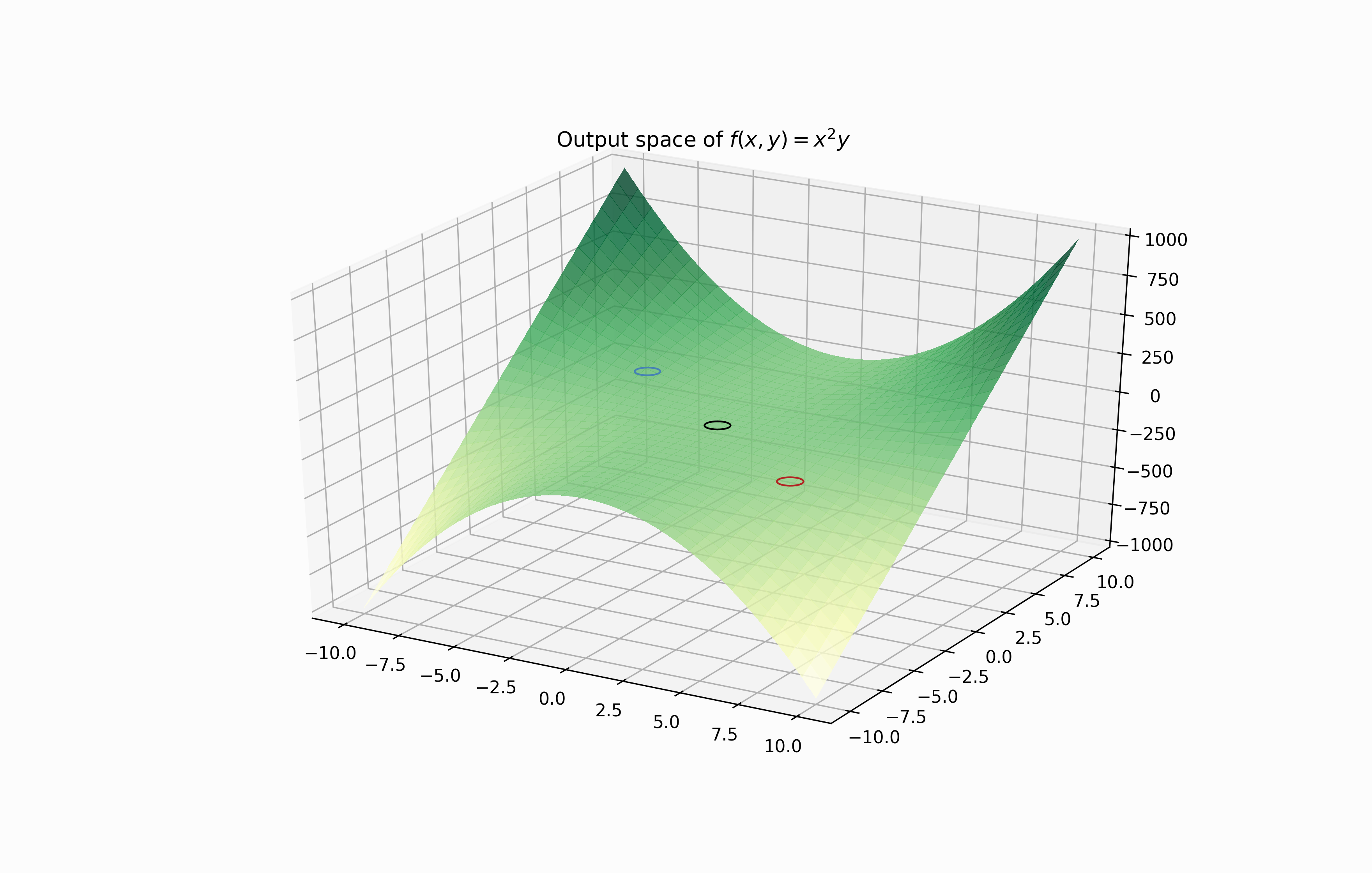
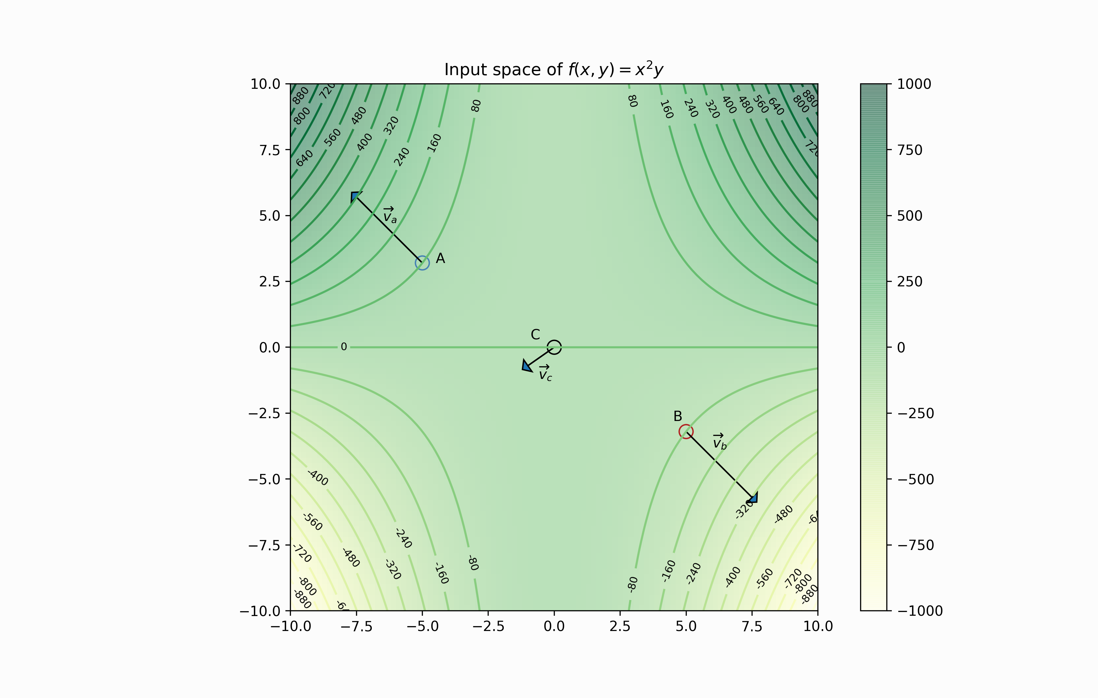
A surface plot will show the output space, and a contour plot the input space of $f (x, y) = x^{2} y$ . We will compute the directional derivatives for three points and their respective directional vectors.

Look the directional vectors in the plot, or tangent vectors as JAX refers to them, there are of different lengths. It's important to remark that if we want the "slope definition" for directional derivatives we need to transform $𝐯$ in a unit length vector (divide the directional derivative definition by $| | v | |$ ). Remember that partial derivatives are computed using unit vectors ( $e_{i}$ ).

\nabla_{𝐯} f = \frac{\partial f}{\partial 𝐱} = l i m_{h \to 0} \frac{f (𝐱 + h 𝐯) - f (𝐱)}{h | | 𝐯 | |}

primal_a = jnp.array([-5., 3.2])
primal_b = jnp.array([5., -3.2])
primal_c = jnp.array([0., 0.])
va = jnp.array([-7.5, 5.7])
vb = jnp.array([7.5, -5.7])
vc = jnp.array([-1.0, -0.7])
unit_va = va/va.dot(va)**.5
unit_vb = vb/vb.dot(vb)**.5
unit_vc = vc/vc.dot(vc)**.5
# Computing making the directional vectors unit length
_, slope_a = jax.jvp(fun, primal_a.tolist(), unit_va.tolist())
_, slope_b = jax.jvp(fun, primal_b.tolist(), unit_vb.tolist())
_, slope_c = jax.jvp(fun, primal_c.tolist(), unit_vc.tolist())
slope_a, slope_b, slope_c
> (DeviceArray(40.60427, dtype=float32, weak_type=True),
   DeviceArray(-40.60427, dtype=float32, weak_type=True),
   DeviceArray(-0., dtype=float32, weak_type=True))

We can see some observations from the points and their directional derivatives.

Point A: the directional derivative is 40.6, makes sense with the contour lines in front of A. The surface start to rise in the direction of ${\vec{v}}_{a}$ .
Point B: the function 𝑓 decreases in the direction pointing out the vector ${\vec{v}}_{b}$ , like the directional derivative, 𝑓 changes −40.6 regarding the slight variations in the input across the directional vector. Notice that it has the same magnitude as the slope of point A but goes in the opposite direction; the surface plot shows how the function increases/decreases in the same proportion across its diagonals.
Point C: the surface is practically flat around the point (0,0). Notice that the directional derivative at ${\vec{v}}_{c}$ is 0.